2 NVMe SSD Comparison: Micron 14T vs WD 14T
Comprehensive fio Benchmark Analysis
2.1 Executive Summary
This report compares two enterprise NVMe SSDs using comprehensive fio benchmarks across various workload profiles. The drives tested are:
- Micron 14T: 14TB capacity, priced at ₹2.2L
- WD 14T: 14TB capacity, priced at ₹1.4L
2.1.1 Key Findings
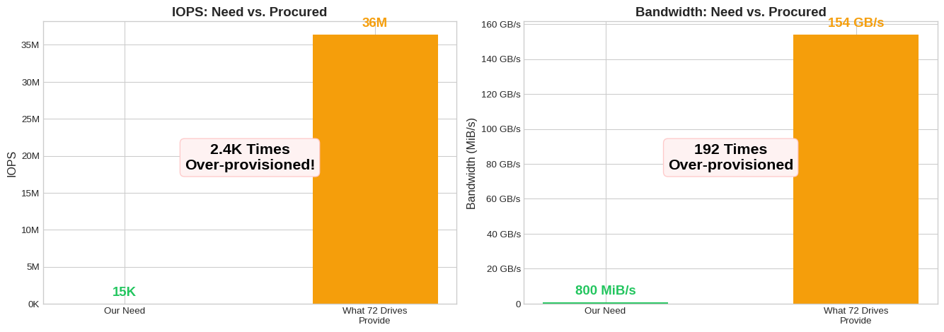
Bottom Line: We are Capacity-Bound, Not Performance-Bound
Neither SSD’s performance matters — our 15K IOPS need is dwarfed by even a single drive’s 505K capability.
The real question: Do we need 1 PB of SSD at all? A tiered SSD+HDD strategy could save significantly more than the Micron vs WD debate.
Why? We need 72 drives to store 1 PB. But those 72 drives deliver 2.4Kx more IOPS and 192x more bandwidth than we actually need.
2.1.2 Our Requirements & Assumptions
Storage Requirements (from production data)
| Requirement | Value | Source |
|---|---|---|
| Total Capacity | ~1 PB | |
| Peak Read IOPS | ~15K | Sum across all DB clusters |
| Peak Write IOPS | ~6K | Clickhouse-logs-cluster peak |
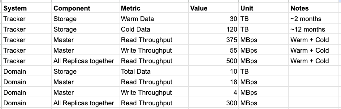
| Read Throughput | ~800 MiB/s | Tracker (500) + Domain (300) all replicas |
| Write Throughput | ~60 MiB/s | Tracker (55) + Domain (4) masters |
| Metric | Micron 14T | WD 14T | Winner |
|---|---|---|---|
| Cost for 1 PB | ₹1.58 Cr (72 drives) | ₹1.0 Cr (72 drives) | WD saves ₹0.58 Cr |
| ₹ per 1K Write IOPS | ₹302 | ₹277 | WD 9% cheaper |
| ₹ per GB/s Write BW | ₹42K | ₹65K | Micron |
| Total IOPS (1 PB) | 52M IOPS | 36M IOPS | Both 2.4Kx overkill |
2.1.3 The Real Insight: Capacity vs Performance
| Metric | Our Need | Single WD Drive | Drives Required | Headroom (72 drives) |
|---|---|---|---|---|
| Capacity | 1 PB | 14 TB | 72 | 1x (bottleneck) |
| IOPS | 15K | 505K | 1 | 2.4Kx |
| Bandwidth | 800 MiB/s | 2.1 GB/s | 1 | 192x |
We need 72 drives for capacity, but only 1 drive worth of IOPS. This screams for a tiered storage architecture.
2.1.4 Quick Facts
- Micron is faster — 1.4-2.4x in write benchmarks
- WD is 1.57x cheaper per TB — ₹10K/TB vs ₹15.7K/TB
- WD is slightly cheaper per IOPS — ₹277 vs ₹302 per 1K IOPS
- Our workload needs ~15K IOPS — a single WD drive does 505K IOPS
- 1 PB with either = 72 drives — WD: 36M IOPS, Micron: 52M IOPS (both overkill)
2.1.5 Strategic Recommendation
Consider SSD+HDD Tiering
Since we’re capacity-bound, not IOPS-bound:
- Hot Tier (SSD): 40-100 TB on WD 14T for active/warm data (3-7 drives)
- Handles all 15K IOPS easily
- Cost: ₹4-10L
- Cold Tier (HDD): 900-960 TB on enterprise HDD (~₹1.5K/TB)
- Archives, cold data, backups
- Cost: ₹13-15L
- Total: ~₹17-25L vs ₹1.0 Cr (all-SSD) = Save ₹75-83L
This is where the real savings are — not in Micron vs WD.
2.2 Key Results
Show code
# Pivot data for side-by-side comparison
key_tests = [
    'iops_randwrite_4k_qd32',
    'iops_randread_4k_qd32',
    'maxiops_randwrite_4k_qd128',
    'maxiops_randread_4k_qd128',
    'throughput_seqwrite_1m',
    'throughput_seqread_1m',
    'mysql_write_16k_qd32',
    'postgres_write_8k_qd32',
    'ceph_write_4k_qd64'
]

results = []
for test in key_tests:
    micron_row = df[(df['test_name'] == test) & (df['drive'] == 'micron_3T')]
    wd_row = df[(df['test_name'] == test) & (df['drive'] == 'wd_14T')]

    if micron_row.empty or wd_row.empty:
        continue

    # Determine primary metric
    if 'write' in test or micron_row['workload_type'].values[0] in ['randwrite', 'write']:
        metric = 'Write IOPS' if 'iops' in test.lower() or 'write' in test.lower() else 'Write BW (MiB/s)'
        micron_val = micron_row['write_iops'].values[0] if pd.notna(micron_row['write_iops'].values[0]) else micron_row['write_bandwidth_mib'].values[0]
        wd_val = wd_row['write_iops'].values[0] if pd.notna(wd_row['write_iops'].values[0]) else wd_row['write_bandwidth_mib'].values[0]
        higher_better = True
    else:
        metric = 'Read IOPS' if 'iops' in test.lower() else 'Read BW (MiB/s)'
        micron_val = micron_row['read_iops'].values[0] if pd.notna(micron_row['read_iops'].values[0]) else micron_row['read_bandwidth_mib'].values[0]
        wd_val = wd_row['read_iops'].values[0] if pd.notna(wd_row['read_iops'].values[0]) else wd_row['read_bandwidth_mib'].values[0]
        higher_better = True

    ratio = micron_val / wd_val if wd_val else 0
    winner = get_winner(micron_val, wd_val, higher_better)

    results.append({
        'Test': test.replace('_', ' ').title(),
        'Metric': metric,
        'Micron 14T': f"{micron_val:,.0f}",
        'WD 14T': f"{wd_val:,.0f}",
        'Ratio (M/W)': f"{ratio:.2f}x",
        'Winner': winner
    })

key_results_df = pd.DataFrame(results)
key_results_df| Test | Metric | Micron 14T | WD 14T | Ratio (M/W) | Winner | |
|---|---|---|---|---|---|---|
| 0 | Iops Randwrite 4K Qd32 | Write IOPS | 729,000 | 505,000 | 1.44x | Micron |
| 1 | Iops Randread 4K Qd32 | Read IOPS | 733,000 | 554,000 | 1.32x | Micron |
| 2 | Maxiops Randwrite 4K Qd128 | Write IOPS | 786,000 | 494,000 | 1.59x | Micron |
| 3 | Maxiops Randread 4K Qd128 | Read IOPS | 1,138,000 | 993,000 | 1.15x | Micron |
| 4 | Throughput Seqwrite 1M | Write IOPS | 5,204 | 2,137 | 2.44x | Micron |
| 5 | Throughput Seqread 1M | Read BW (MiB/s) | 6,306 | 4,850 | 1.30x | Micron |
| 6 | Mysql Write 16K Qd32 | Write IOPS | 267,000 | 136,000 | 1.96x | Micron |
| 7 | Postgres Write 8K Qd32 | Write IOPS | 432,000 | 266,000 | 1.62x | Micron |
| 8 | Ceph Write 4K Qd64 | Write IOPS | 785,000 | 504,000 | 1.56x | Micron |
2.3 Tail Latency Analysis
Tail latency (p99 and above) is critical for database and latency-sensitive workloads. Lower values indicate more consistent performance.
Show code
tail_tests = [
    ('iops_randwrite_4k_qd32', 'write'),
    ('iops_randread_4k_qd32', 'read'),
    ('mysql_write_16k_qd32', 'write'),
    ('postgres_write_8k_qd32', 'write'),
    ('ceph_write_4k_qd64', 'write'),
    ('randwrite_8k_qd32', 'write'),
    ('randread_8k_qd32', 'read')
]

tail_results = []
for test, op_type in tail_tests:
    micron_row = df[(df['test_name'] == test) & (df['drive'] == 'micron_3T')]
    wd_row = df[(df['test_name'] == test) & (df['drive'] == 'wd_14T')]

    if micron_row.empty or wd_row.empty:
        continue

    prefix = f"{op_type}_"

    micron_p99 = micron_row[f'{prefix}p99_latency_us'].values[0]
    wd_p99 = wd_row[f'{prefix}p99_latency_us'].values[0]
    micron_p99_9 = micron_row[f'{prefix}p99_9_latency_us'].values[0]
    wd_p99_9 = wd_row[f'{prefix}p99_9_latency_us'].values[0]

    p99_winner = get_winner(micron_p99, wd_p99, higher_is_better=False)

    tail_results.append({
        'Test': test.replace('_', ' ').title(),
        'Operation': op_type.capitalize(),
        'Micron p99 (µs)': f"{micron_p99:,.0f}" if pd.notna(micron_p99) else "N/A",
        'WD p99 (µs)': f"{wd_p99:,.0f}" if pd.notna(wd_p99) else "N/A",
        'Micron p99.9 (µs)': f"{micron_p99_9:,.0f}" if pd.notna(micron_p99_9) else "N/A",
        'WD p99.9 (µs)': f"{wd_p99_9:,.0f}" if pd.notna(wd_p99_9) else "N/A",
        'p99 Winner': p99_winner
    })

tail_df = pd.DataFrame(tail_results)
tail_df| Test | Operation | Micron p99 (µs) | WD p99 (µs) | Micron p99.9 (µs) | WD p99.9 (µs) | p99 Winner | |
|---|---|---|---|---|---|---|---|
| 0 | Iops Randwrite 4K Qd32 | Write | 192 | 412 | 225 | 570 | Micron |
| 1 | Iops Randread 4K Qd32 | Read | 302 | 660 | 400 | 922 | Micron |
| 2 | Mysql Write 16K Qd32 | Write | 1,139 | 2,311 | 1,614 | 5,735 | Micron |
| 3 | Postgres Write 8K Qd32 | Write | 750 | 1,336 | 807 | 1,729 | Micron |
| 4 | Ceph Write 4K Qd64 | Write | 668 | 1,516 | 717 | 1,827 | Micron |
| 5 | Randwrite 8K Qd32 | Write | 469 | 717 | 498 | 930 | Micron |
| 6 | Randread 8K Qd32 | Read | 441 | 523 | 594 | 750 | Micron |
Observations:
- Micron shows significantly tighter p99 latencies in write workloads (often 50% lower)
- WD’s p99.9 latencies can spike dramatically under write pressure (14ms+ in Postgres write vs 938µs for Micron)
- For read-heavy workloads, the gap narrows considerably
2.4 Sequential Bandwidth
Show code
seq_tests = [
    'throughput_seqwrite_1m',
    'throughput_seqread_1m',
    'largefile_seqwrite_4m',
    'largefile_seqread_4m',
    'kafka_seqwrite_64k'
]

seq_results = []
for test in seq_tests:
    micron_row = df[(df['test_name'] == test) & (df['drive'] == 'micron_3T')]
    wd_row = df[(df['test_name'] == test) & (df['drive'] == 'wd_14T')]

    if micron_row.empty or wd_row.empty:
        continue

    is_write = 'write' in test

    if is_write:
        micron_bw = micron_row['write_bandwidth_mib'].values[0]
        wd_bw = wd_row['write_bandwidth_mib'].values[0]
    else:
        micron_bw = micron_row['read_bandwidth_mib'].values[0]
        wd_bw = wd_row['read_bandwidth_mib'].values[0]

    ratio = micron_bw / wd_bw if wd_bw else 0
    winner = get_winner(micron_bw, wd_bw, higher_is_better=True)

    seq_results.append({
        'Test': test.replace('_', ' ').title(),
        'Block Size': '1M' if '1m' in test else ('4M' if '4m' in test else '64K'),
        'Operation': 'Write' if is_write else 'Read',
        'Micron (MiB/s)': f"{micron_bw:,.0f}",
        'WD (MiB/s)': f"{wd_bw:,.0f}",
        'Ratio': f"{ratio:.2f}x",
        'Winner': winner
    })

seq_df = pd.DataFrame(seq_results)
seq_df| Test | Block Size | Operation | Micron (MiB/s) | WD (MiB/s) | Ratio | Winner | |
|---|---|---|---|---|---|---|---|
| 0 | Throughput Seqwrite 1M | 1M | Write | 5,204 | 2,137 | 2.44x | Micron |
| 1 | Throughput Seqread 1M | 1M | Read | 6,307 | 4,850 | 1.30x | Micron |
| 2 | Largefile Seqwrite 4M | 4M | Write | 5,196 | 2,131 | 2.44x | Micron |
| 3 | Largefile Seqread 4M | 4M | Read | 6,333 | 4,768 | 1.33x | Micron |
| 4 | Kafka Seqwrite 64K | 64K | Write | 5,132 | 2,124 | 2.42x | Micron |
Inference: The dramatic sequential write difference (2.4x for 1M blocks) suggests Micron may be using PCIe Gen4 or has significantly better controller/firmware optimization for sustained writes. WD appears to throttle heavily under sustained sequential write pressure.
2.5 Database-like Workloads
Show code
db_tests = [
    'mysql_write_16k_qd32',
    'mysql_read_16k_qd32',
    'mysql_mixed_16k_qd32',
    'postgres_write_8k_qd32',
    'postgres_read_8k_qd32',
    'postgres_mixed_8k_qd32'
]

db_results = []
for test in db_tests:
    micron_row = df[(df['test_name'] == test) & (df['drive'] == 'micron_3T')]
    wd_row = df[(df['test_name'] == test) & (df['drive'] == 'wd_14T')]

    if micron_row.empty or wd_row.empty:
        continue

    db_type = 'MySQL' if 'mysql' in test else 'PostgreSQL'
    workload = 'Write' if 'write' in test else ('Read' if 'read' in test else 'Mixed')

    # Get primary metric based on workload
    if workload == 'Write':
        micron_iops = micron_row['write_iops'].values[0]
        wd_iops = wd_row['write_iops'].values[0]
        micron_lat = micron_row['write_p50_latency_us'].values[0]
        wd_lat = wd_row['write_p50_latency_us'].values[0]
    elif workload == 'Read':
        micron_iops = micron_row['read_iops'].values[0]
        wd_iops = wd_row['read_iops'].values[0]
        micron_lat = micron_row['read_p50_latency_us'].values[0]
        wd_lat = wd_row['read_p50_latency_us'].values[0]
    else:  # Mixed - report both
        micron_iops = micron_row['read_iops'].values[0] + micron_row['write_iops'].values[0]
        wd_iops = wd_row['read_iops'].values[0] + wd_row['write_iops'].values[0]
        micron_lat = micron_row['write_p50_latency_us'].values[0]  # Focus on write latency for mixed
        wd_lat = wd_row['write_p50_latency_us'].values[0]

    ratio = micron_iops / wd_iops if wd_iops else 0

    db_results.append({
        'Database': db_type,
        'Workload': workload,
        'Micron IOPS': f"{micron_iops:,.0f}",
        'WD IOPS': f"{wd_iops:,.0f}",
        'Ratio': f"{ratio:.2f}x",
        'Micron p50 (µs)': f"{micron_lat:,.0f}" if pd.notna(micron_lat) else "N/A",
        'WD p50 (µs)': f"{wd_lat:,.0f}" if pd.notna(wd_lat) else "N/A",
        'Winner': 'Micron' if ratio > 1 else 'WD'
    })

db_df = pd.DataFrame(db_results)
db_df| Database | Workload | Micron IOPS | WD IOPS | Ratio | Micron p50 (µs) | WD p50 (µs) | Winner | |
|---|---|---|---|---|---|---|---|---|
| 0 | MySQL | Write | 267,000 | 136,000 | 1.96x | 938 | 1,844 | Micron |
| 1 | MySQL | Read | 391,000 | 336,000 | 1.16x | 570 | 652 | Micron |
| 2 | MySQL | Mixed | 571,000 | 337,000 | 1.69x | 1,319 | 668 | Micron |
| 3 | PostgreSQL | Write | 432,000 | 266,000 | 1.62x | 586 | 930 | Micron |
| 4 | PostgreSQL | Read | 704,000 | 610,000 | 1.15x | 359 | 396 | Micron |
| 5 | PostgreSQL | Mixed | 861,000 | 588,000 | 1.46x | 889 | 424 | Micron |
Key Insight: For database workloads, Micron’s advantage is most pronounced in write-heavy scenarios:
- PostgreSQL write: 1.6x more IOPS with 37% lower latency
- MySQL write: 2.0x more IOPS with 49% lower latency
- Mixed workloads show Micron handling concurrent read+write pressure better
2.6 Cost & Value Analysis
Show code
# 1 PB deployment calculations
TARGET_CAPACITY_TB = 1000  # 1 PB

# Drives needed
wd_drives_for_1pb = int(np.ceil(TARGET_CAPACITY_TB / CAPACITY_WD))
micron_drives_for_1pb = int(np.ceil(TARGET_CAPACITY_TB / CAPACITY_MICRON))

# Total cost
wd_cost_1pb = wd_drives_for_1pb * PRICE_WD_14T
micron_cost_1pb = micron_drives_for_1pb * PRICE_MICRON_14T

# Total IOPS capacity (using QD32 random write as baseline)
wd_total_iops = wd_drives_for_1pb * rw_qd32_wd
micron_total_iops = micron_drives_for_1pb * rw_qd32_micron

# Total sequential write bandwidth
wd_total_bw = wd_drives_for_1pb * seq_write_wd
micron_total_bw = micron_drives_for_1pb * seq_write_micron

# Cost per IOPS (per 1K IOPS)
wd_cost_per_kiops = PRICE_WD_14T / (rw_qd32_wd / 1000)
micron_cost_per_kiops = PRICE_MICRON_14T / (rw_qd32_micron / 1000)

# Calculate cost metrics table
cost_data = {
    'Metric': [
        'Price per drive',
        'Capacity per drive',
        '**Price per TB**',
        '**₹ per 1K Write IOPS**',
        '₹ per GB/s Seq Write',
        'Drives for 1 PB',
        '**Total cost for 1 PB**',
        'Total Write IOPS (1 PB)',
        'Total Seq Write BW (1 PB)'
    ],
    'Micron 14T': [
        format_inr(PRICE_MICRON_14T),
        f'{CAPACITY_MICRON} TB',
        format_inr(PRICE_PER_TB_MICRON),
        f'₹{micron_cost_per_kiops:,.0f}',
        f'₹{PRICE_MICRON_14T / (seq_write_micron/1000):,.0f}',
        f'{micron_drives_for_1pb}',
        f'₹{micron_cost_1pb/10000000:.1f} Cr',
        f'{micron_total_iops/1000000:.0f}M IOPS',
        f'{micron_total_bw/1000:.0f} GB/s'
    ],
    'WD 14T': [
        format_inr(PRICE_WD_14T),
        f'{CAPACITY_WD} TB',
        format_inr(PRICE_PER_TB_WD),
        f'₹{wd_cost_per_kiops:,.0f}',
        f'₹{PRICE_WD_14T / (seq_write_wd/1000):,.0f}',
        f'{wd_drives_for_1pb}',
        f'₹{wd_cost_1pb/10000000:.1f} Cr',
        f'{wd_total_iops/1000000:.0f}M IOPS',
        f'{wd_total_bw/1000:.0f} GB/s'
    ],
    'Winner': [
        'WD (₹80K cheaper)',
        'Equal (14 TB each)',
        '**WD (1.57x cheaper)**',
        '**WD (9% cheaper)**',
        'Micron (1.5x)',
        'Equal (72 drives each)',
        '**WD saves ₹0.58 Cr**',
        'Micron (1.4x)',
        'Micron (2.4x)'
    ]
}

cost_df = pd.DataFrame(cost_data)
cost_df| Metric | Micron 14T | WD 14T | Winner | |
|---|---|---|---|---|
| 0 | Price per drive | ₹2.20L | ₹1.40L | WD (₹80K cheaper) |
| 1 | Capacity per drive | 14 TB | 14 TB | Equal (14 TB each) |
| 2 | **Price per TB** | ₹15.7K | ₹10.0K | **WD (1.57x cheaper)** |
| 3 | **₹ per 1K Write IOPS** | ₹302 | ₹277 | **WD (9% cheaper)** |
| 4 | ₹ per GB/s Seq Write | ₹42,275 | ₹65,512 | Micron (1.5x) |
| 5 | Drives for 1 PB | 72 | 72 | Equal (72 drives each) |
| 6 | **Total cost for 1 PB** | ₹1.6 Cr | ₹1.0 Cr | **WD saves ₹0.58 Cr** |
| 7 | Total Write IOPS (1 PB) | 52M IOPS | 36M IOPS | Micron (1.4x) |
| 8 | Total Seq Write BW (1 PB) | 375 GB/s | 154 GB/s | Micron (2.4x) |
2.6.1 The Money Shot: 1 PB Deployment
Show code
fig, axes = plt.subplots(1, 3, figsize=(14, 5))

# Chart 1: Total Cost
ax1 = axes[0]
costs = [micron_cost_1pb/10000000, wd_cost_1pb/10000000]
bars1 = ax1.bar(['Micron', 'WD'], costs, color=[MICRON_COLOR, WD_COLOR])
ax1.set_ylabel('Cost (₹ Crores)', fontsize=12)
ax1.set_title('Total Cost for 1 PB', fontsize=13, fontweight='bold')
for bar, val in zip(bars1, costs):
    ax1.annotate(f'₹{val:.1f} Cr', xy=(bar.get_x() + bar.get_width()/2, bar.get_height()),
                ha='center', va='bottom', fontsize=12, fontweight='bold')
ax1.annotate(f'Saves\n₹{(micron_cost_1pb-wd_cost_1pb)/10000000:.1f} Cr',
             xy=(1, costs[1] + 0.5), ha='center', fontsize=11, color='#059669', fontweight='bold')

# Chart 2: Number of Drives
ax2 = axes[1]
drives = [micron_drives_for_1pb, wd_drives_for_1pb]
bars2 = ax2.bar(['Micron', 'WD'], drives, color=[MICRON_COLOR, WD_COLOR])
ax2.set_ylabel('Number of Drives', fontsize=12)
ax2.set_title('Drives Required for 1 PB', fontsize=13, fontweight='bold')
for bar, val in zip(bars2, drives):
    ax2.annotate(f'{val}', xy=(bar.get_x() + bar.get_width()/2, bar.get_height()),
                ha='center', va='bottom', fontsize=12, fontweight='bold')

# Chart 3: Cost per IOPS
ax3 = axes[2]
cost_per_iops = [micron_cost_per_kiops, wd_cost_per_kiops]
bars3 = ax3.bar(['Micron', 'WD'], cost_per_iops, color=[MICRON_COLOR, WD_COLOR])
ax3.set_ylabel('₹ per 1K Write IOPS', fontsize=12)
ax3.set_title('Cost Efficiency (Lower = Better)', fontsize=13, fontweight='bold')
for bar, val in zip(bars3, cost_per_iops):
    ax3.annotate(f'₹{val:.0f}', xy=(bar.get_x() + bar.get_width()/2, bar.get_height()),
                ha='center', va='bottom', fontsize=12, fontweight='bold')
ax3.annotate(f'9%\ncheaper', xy=(1, cost_per_iops[1] + 30), ha='center', fontsize=11,
             color='#059669', fontweight='bold')

plt.tight_layout()
plt.show()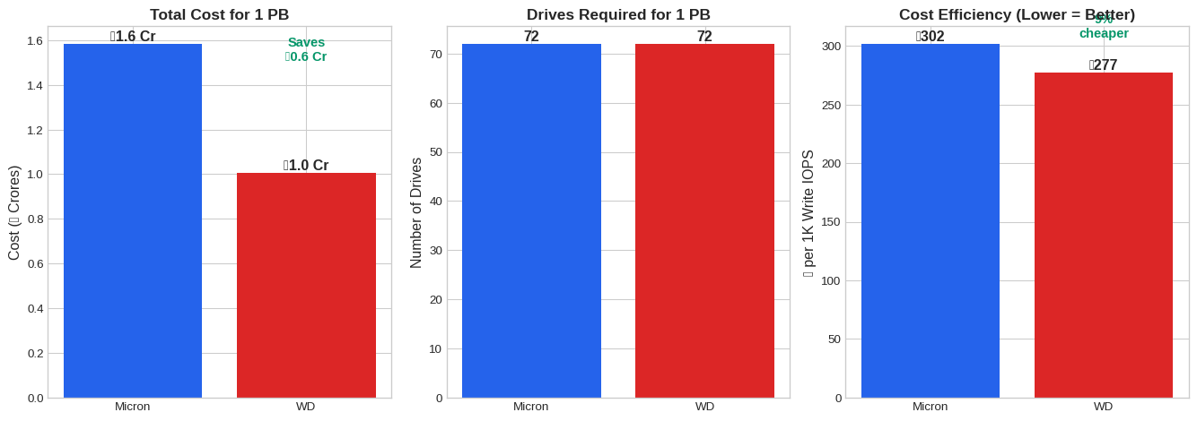
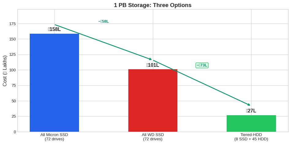
2.6.2 But Wait: What About HDD?
Since we’re capacity-bound (not IOPS-bound), there’s a bigger cost lever: SSD+HDD tiering.
| Storage | Price/TB | Write IOPS | Use Case | |
|---|---|---|---|---|
| 0 | WD 14T SSD | ₹10K | 505K | Hot data |
| 1 | Seagate 20T HDD | ₹1.7K | 350 | Cold archives |
| 2 | Ratio | **SSD 5.8x costlier** | **SSD 1,443x faster** | — |
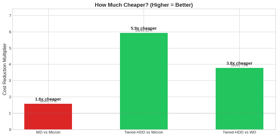
Key Insight: Tiering is the Bigger Lever
| Comparison | Multiplier | Savings |
|---|---|---|
| Micron → WD | 1.6x cheaper | ₹58L (37%) |
| Micron → Tiered-HDD | 5.9x cheaper | ₹131L (83%) |
| WD → Tiered-HDD | 3.7x cheaper | ₹73L (73%) |
The Micron vs WD debate (1.6x) matters far less than the SSD vs Tiered-HDD decision (3.7-5.9x). See Appendix A: SSD+HDD Tiering Analysis for detailed calculations.
2.7 Real-World Workload Analysis
Our actual storage requirements from production clusters:
Show code
# Our actual requirements (from db-traffic.png)
ACTUAL_READ_THROUGHPUT_MBPS = 500 + 300  # Tracker + Domain all replicas
ACTUAL_WRITE_THROUGHPUT_MBPS = 55 + 4    # Tracker + Domain master
ACTUAL_STORAGE_WARM_TB = 30 + 10         # Warm data
ACTUAL_STORAGE_COLD_TB = 120             # Cold data

# Load AWS cluster data
cluster_df = pd.read_csv('Server - AWS Instance Distribution - IO Throughput Across Clusters.csv',
                          skiprows=1)
cluster_df.columns = ['cluster', 'volumes', 'capacity_gib', 'read_ops', 'write_ops',
                      'read_throughput_gib', 'write_throughput_gib', 'avg_read_iops', 'avg_write_iops']

# Clean numeric columns
for col in ['avg_read_iops', 'avg_write_iops', 'read_throughput_gib', 'write_throughput_gib']:
    cluster_df[col] = pd.to_numeric(cluster_df[col], errors='coerce')

# Calculate totals
total_read_iops = cluster_df['avg_read_iops'].sum()
total_write_iops = cluster_df['avg_write_iops'].sum()
total_read_bw = cluster_df['read_throughput_gib'].sum()  # Already in GiB for 7 days
total_write_bw = cluster_df['write_throughput_gib'].sum()

# Peak values (single cluster max)
peak_write_iops = cluster_df['avg_write_iops'].max()
peak_cluster = cluster_df.loc[cluster_df['avg_write_iops'].idxmax(), 'cluster']

print(f"Peak write IOPS: {peak_write_iops:,.0f} ({peak_cluster})")
Peak write IOPS: 6,187 (clickhouse-logs-cluster)2.7.1 Actual vs Available IOPS
Show code
# Conservative estimates for our workload
our_peak_iops = 15000  # ~15K IOPS peak from cluster data
our_avg_bw_mbps = 800  # ~800 MiB/s combined read+write

fig, axes = plt.subplots(1, 2, figsize=(12, 5))

# IOPS comparison
ax1 = axes[0]
iops_data = [our_peak_iops/1000, wd_total_iops/1000000 * 1000]  # Convert to same scale (K)
colors = ['#f59e0b', WD_COLOR]
bars = ax1.bar(['Our Peak Need', f'WD 1PB Capacity\n({wd_drives_for_1pb} drives)'],
               [our_peak_iops, wd_total_iops], color=colors)
ax1.set_ylabel('Write IOPS', fontsize=12)
ax1.set_title('IOPS: Need vs Capacity', fontsize=13, fontweight='bold')
ax1.set_yscale('log')
ax1.annotate(f'{our_peak_iops/1000:.0f}K', xy=(0, our_peak_iops), ha='center', va='bottom',
             fontsize=12, fontweight='bold')
ax1.annotate(f'{wd_total_iops/1000000:.0f}M', xy=(1, wd_total_iops), ha='center', va='bottom',
             fontsize=12, fontweight='bold')
headroom = wd_total_iops / our_peak_iops
ax1.annotate(f'{headroom/1000:.1f}Kx\nheadroom!', xy=(0.5, np.sqrt(our_peak_iops * wd_total_iops)),
             ha='center', fontsize=14, color='#059669', fontweight='bold')

# Bandwidth comparison
ax2 = axes[1]
bw_data = [our_avg_bw_mbps, wd_total_bw]
bars2 = ax2.bar(['Our Need', f'WD 1PB Capacity'], bw_data, color=colors)
ax2.set_ylabel('Bandwidth (MiB/s)', fontsize=12)
ax2.set_title('Seq Write BW: Need vs Capacity', fontsize=13, fontweight='bold')
ax2.annotate(f'{our_avg_bw_mbps:,} MiB/s', xy=(0, our_avg_bw_mbps), ha='center', va='bottom',
             fontsize=12, fontweight='bold')
ax2.annotate(f'{wd_total_bw/1000:.0f} GB/s', xy=(1, wd_total_bw), ha='center', va='bottom',
             fontsize=12, fontweight='bold')
bw_headroom = wd_total_bw / our_avg_bw_mbps
ax2.annotate(f'{bw_headroom:.0f}x\nheadroom', xy=(0.5, (our_avg_bw_mbps + wd_total_bw)/2),
             ha='center', fontsize=14, color='#059669', fontweight='bold')

plt.tight_layout()
plt.show()
2.7.2 Cluster-by-Cluster IOPS Analysis
Show code
# Show top clusters by write IOPS
top_clusters = cluster_df.nlargest(10, 'avg_write_iops')[['cluster', 'volumes', 'avg_write_iops', 'avg_read_iops']].copy()
top_clusters['avg_write_iops'] = top_clusters['avg_write_iops'].apply(lambda x: f"{x:,.0f}")
top_clusters['avg_read_iops'] = top_clusters['avg_read_iops'].apply(lambda x: f"{x:,.0f}")
top_clusters.columns = ['Cluster', 'Volumes', 'Avg Write IOPS', 'Avg Read IOPS']
top_clusters| Cluster | Volumes | Avg Write IOPS | Avg Read IOPS | |
|---|---|---|---|---|
| 9 | clickhouse-logs-cluster | 24 | 6,187 | 978 |
| 18 | advance-opensearch | 17 | 2,821 | 2,559 |
| 31 | clickhouse-kv-cluster | 12 | 2,092 | 766 |
| 24 | euler-kafka-broker-o2 | 24 | 1,992 | 451 |
| 35 | ckh-server-sdk | 9 | 1,462 | 35 |
| 30 | vlogs | 11 | 1,074 | 1,337 |
| 11 | cassandra-kv-sessionizer | 20 | 975 | 6,380 |
| 5 | clickhouse-keeper | 18 | 958 | 19 |
| 16 | ckh-keeper-sdk | 9 | 796 | 0 |
| 7 | kafkabroker | 36 | 663 | 5 |
2.7.3 Summary: We’re Massively Over-Provisioned on IOPS
Show code
summary_data = {
    'Metric': [
        'Our Peak Write IOPS',
        'Single WD Drive',
        'WD Capacity (72 drives for 1 PB)',
        '**Headroom Factor**',
        '',
        'Our Peak Bandwidth',
        'Single WD Drive',
        'WD Capacity (72 drives)',
        '**Headroom Factor**'
    ],
    'Value': [
        '~15K IOPS',
        '505K IOPS',
        '36M IOPS',
        f'**{wd_total_iops/15000/1000:.1f}Kx**',
        '',
        '~800 MiB/s',
        '2.1 GB/s',
        f'{wd_total_bw/1000:.0f} GB/s',
        f'**{int(wd_total_bw/800)}x**'
    ],
    'Notes': [
        'Sum across all production clusters',
        'At QD32 random write',
        'Linear scaling (conservative)',
        '2.4Kx more than we need',
        '',
        'Combined read + write',
        'Sequential 1M writes',
        'Linear scaling',
        '~190x more than we need'
    ]
}

summary_df = pd.DataFrame(summary_data)
summary_df| Metric | Value | Notes | |
|---|---|---|---|
| 0 | Our Peak Write IOPS | ~15K IOPS | Sum across all production clusters |
| 1 | Single WD Drive | 505K IOPS | At QD32 random write |
| 2 | WD Capacity (72 drives for 1 PB) | 36M IOPS | Linear scaling (conservative) |
| 3 | **Headroom Factor** | **2.4Kx** | 2.4Kx more than we need |
| 4 | |||
| 5 | Our Peak Bandwidth | ~800 MiB/s | Combined read + write |
| 6 | Single WD Drive | 2.1 GB/s | Sequential 1M writes |
| 7 | WD Capacity (72 drives) | 154 GB/s | Linear scaling |
| 8 | **Headroom Factor** | **192x** | ~190x more than we need |
Recommendation: Tiered-HDD Storage Strategy
Don’t choose between Micron and WD for 1 PB — choose tiering instead.
| Tier | Storage | Capacity | Drives | Cost | Purpose |
|---|---|---|---|---|---|
| Hot | WD 14T SSD | 56-84 TB | 4-6 | ₹5.6-8.4L | Active data, all I/O |
| Cold | Enterprise HDD | ~920 TB | ~46 | ₹13-14L | Archives, cold data |
| Total | 1 PB | ~50-52 | ₹18-22L |
vs All-SSD (WD): 72 drives, ₹1.0 Cr → Save ₹78-82L with tiering
The 4-6 SSDs in the hot tier provide:
- 2-3M IOPS (vs our 15K need = 130-200x headroom)
- 8.5-12.8 GB/s bandwidth (vs our 800 MiB/s need = 10-16x headroom)
2.7.4 When Would All-SSD Make Sense?
| Scenario | Threshold | Our Status |
|---|---|---|
| Random I/O on entire dataset | Need SSD everywhere | ❌ 80%+ data is cold |
| Latency-critical cold reads | Sub-ms required | ❌ HDD 5-10ms is fine for archives |
| Operational simplicity | One tier is simpler | ⚠️ Valid, but ₹80L savings justifies complexity |
| Rapid data tier changes | Hot/cold unpredictable | ❌ Our access patterns are predictable |
2.8 Performance Visualizations
2.8.1 Random Write IOPS Comparison
Show code
tests = ['iops_randwrite_4k_qd32', 'maxiops_randwrite_4k_qd128']
labels = ['4K QD32', '4K QD128']

micron_vals = []
wd_vals = []

for test in tests:
    m = df[(df['test_name'] == test) & (df['drive'] == 'micron_3T')]['write_iops'].values[0]
    w = df[(df['test_name'] == test) & (df['drive'] == 'wd_14T')]['write_iops'].values[0]
    micron_vals.append(m/1000)
    wd_vals.append(w/1000)

x = np.arange(len(labels))
width = 0.35

fig, ax = plt.subplots(figsize=(10, 6))
bars1 = ax.bar(x - width/2, micron_vals, width, label='Micron 14T', color=MICRON_COLOR)
bars2 = ax.bar(x + width/2, wd_vals, width, label='WD 14T', color=WD_COLOR)

ax.set_ylabel('IOPS (thousands)', fontsize=12)
ax.set_title('Random Write IOPS Comparison', fontsize=14, fontweight='bold')
ax.set_xticks(x)
ax.set_xticklabels(labels)
ax.legend()

# Add value labels on bars
for bar, val in zip(bars1, micron_vals):
    ax.annotate(f'{val:.0f}K', xy=(bar.get_x() + bar.get_width()/2, bar.get_height() + 5),
                ha='center', va='bottom', fontsize=10, fontweight='bold')
for bar, val in zip(bars2, wd_vals):
    ax.annotate(f'{val:.0f}K', xy=(bar.get_x() + bar.get_width()/2, bar.get_height() + 5),
                ha='center', va='bottom', fontsize=10, fontweight='bold')

# Add ratio annotations above both bars
for i, (m, w) in enumerate(zip(micron_vals, wd_vals)):
    ratio = m/w
    ax.annotate(f'{ratio:.1f}x', xy=(x[i], max(m, w) + 80), ha='center', fontsize=11,
                color='#059669', fontweight='bold',
                bbox=dict(boxstyle='round,pad=0.2', facecolor='#ecfdf5', edgecolor='#059669', alpha=0.8))

ax.set_ylim(0, max(max(micron_vals), max(wd_vals)) * 1.25)  # Room for annotations
plt.tight_layout()
plt.show()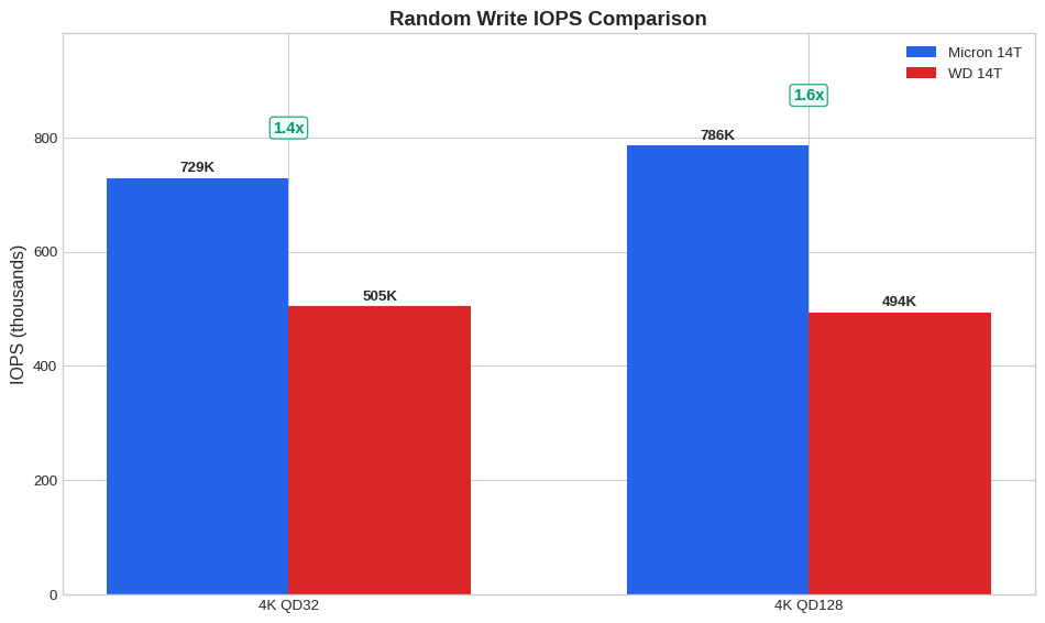
2.8.2 Sequential Write Bandwidth
Show code
tests = ['throughput_seqwrite_1m', 'largefile_seqwrite_4m', 'kafka_seqwrite_64k']
labels = ['1M Block', '4M Block', 'Kafka 64K']

micron_vals = []
wd_vals = []

for test in tests:
    m = df[(df['test_name'] == test) & (df['drive'] == 'micron_3T')]['write_bandwidth_mib'].values[0]
    w = df[(df['test_name'] == test) & (df['drive'] == 'wd_14T')]['write_bandwidth_mib'].values[0]
    micron_vals.append(m)
    wd_vals.append(w)

x = np.arange(len(labels))
width = 0.35

fig, ax = plt.subplots(figsize=(10, 6))
bars1 = ax.bar(x - width/2, micron_vals, width, label='Micron 14T', color=MICRON_COLOR)
bars2 = ax.bar(x + width/2, wd_vals, width, label='WD 14T', color=WD_COLOR)

ax.set_ylabel('Bandwidth (MiB/s)', fontsize=12)
ax.set_title('Sequential Write Bandwidth Comparison', fontsize=14, fontweight='bold')
ax.set_xticks(x)
ax.set_xticklabels(labels)
ax.legend()

# Add value labels on bars
for bar, val in zip(bars1, micron_vals):
    ax.annotate(f'{val:,.0f}', xy=(bar.get_x() + bar.get_width()/2, bar.get_height() + 50),
                ha='center', va='bottom', fontsize=10, fontweight='bold')
for bar, val in zip(bars2, wd_vals):
    ax.annotate(f'{val:,.0f}', xy=(bar.get_x() + bar.get_width()/2, bar.get_height() + 50),
                ha='center', va='bottom', fontsize=10, fontweight='bold')

# Add ratio annotations above both bars
for i, (m, w) in enumerate(zip(micron_vals, wd_vals)):
    ratio = m/w
    ax.annotate(f'{ratio:.1f}x', xy=(x[i], max(m, w) + 400), ha='center', fontsize=11,
                color='#059669', fontweight='bold',
                bbox=dict(boxstyle='round,pad=0.2', facecolor='#ecfdf5', edgecolor='#059669', alpha=0.8))

ax.set_ylim(0, max(max(micron_vals), max(wd_vals)) * 1.25)  # Room for annotations
plt.tight_layout()
plt.show()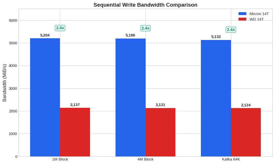
2.8.3 p99 Latency Comparison
Show code
tests = [
    ('iops_randwrite_4k_qd32', 'write', 'RandWrite 4K'),
    ('mysql_write_16k_qd32', 'write', 'MySQL Write'),
    ('postgres_write_8k_qd32', 'write', 'Postgres Write'),
    ('iops_randread_4k_qd32', 'read', 'RandRead 4K')
]

labels = []
micron_vals = []
wd_vals = []

for test, op, label in tests:
    m_row = df[(df['test_name'] == test) & (df['drive'] == 'micron_3T')]
    w_row = df[(df['test_name'] == test) & (df['drive'] == 'wd_14T')]

    m = m_row[f'{op}_p99_latency_us'].values[0]
    w = w_row[f'{op}_p99_latency_us'].values[0]

    if pd.notna(m) and pd.notna(w):
        labels.append(label)
        micron_vals.append(m)
        wd_vals.append(w)

x = np.arange(len(labels))
width = 0.35

fig, ax = plt.subplots(figsize=(10, 6))
bars1 = ax.bar(x - width/2, micron_vals, width, label='Micron 14T', color=MICRON_COLOR)
bars2 = ax.bar(x + width/2, wd_vals, width, label='WD 14T', color=WD_COLOR)

ax.set_ylabel('p99 Latency (µs)', fontsize=12)
ax.set_title('p99 Latency Comparison (Lower is Better)', fontsize=14, fontweight='bold')
ax.set_xticks(x)
ax.set_xticklabels(labels)
ax.legend()

# Add value labels with offset to avoid overlap
max_val = max(max(micron_vals), max(wd_vals))
offset = max_val * 0.02
for bar, val in zip(bars1, micron_vals):
    ax.annotate(f'{val:,.0f}', xy=(bar.get_x() + bar.get_width()/2, bar.get_height() + offset),
                ha='center', va='bottom', fontsize=9, fontweight='bold')
for bar, val in zip(bars2, wd_vals):
    ax.annotate(f'{val:,.0f}', xy=(bar.get_x() + bar.get_width()/2, bar.get_height() + offset),
                ha='center', va='bottom', fontsize=9, fontweight='bold')

ax.set_ylim(0, max_val * 1.15)  # Room for annotations
plt.tight_layout()
plt.show()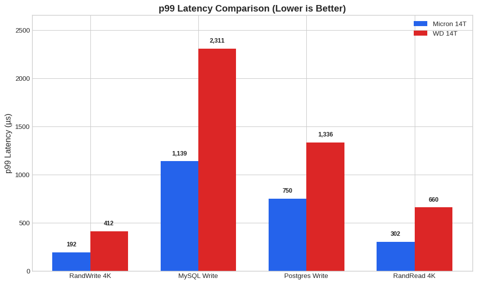
2.8.4 Performance Ratio Across All Tests
Show code
# Calculate ratios for all comparable tests
ratios = []
test_labels = []

for test in df['test_name'].unique():
    m_row = df[(df['test_name'] == test) & (df['drive'] == 'micron_3T')]
    w_row = df[(df['test_name'] == test) & (df['drive'] == 'wd_14T')]

    if m_row.empty or w_row.empty:
        continue

    # Get primary metric
    workload = m_row['workload_type'].values[0]
    if workload in ['randwrite', 'write']:
        m_val = m_row['write_iops'].values[0]
        w_val = w_row['write_iops'].values[0]
        if pd.isna(m_val) or pd.isna(w_val):
            m_val = m_row['write_bandwidth_mib'].values[0]
            w_val = w_row['write_bandwidth_mib'].values[0]
    elif workload in ['randread', 'read']:
        m_val = m_row['read_iops'].values[0]
        w_val = w_row['read_iops'].values[0]
        if pd.isna(m_val) or pd.isna(w_val):
            m_val = m_row['read_bandwidth_mib'].values[0]
            w_val = w_row['read_bandwidth_mib'].values[0]
    else:  # mixed
        m_val = m_row['read_iops'].values[0] + m_row['write_iops'].values[0]
        w_val = w_row['read_iops'].values[0] + w_row['write_iops'].values[0]

    if pd.notna(m_val) and pd.notna(w_val) and w_val > 0:
        ratios.append(m_val / w_val)
        # Shorten test name
        short_name = test.replace('_', ' ').replace('qd', 'Q')
        test_labels.append(short_name[:20])

# Sort by ratio
sorted_pairs = sorted(zip(ratios, test_labels), reverse=True)
ratios, test_labels = zip(*sorted_pairs)

fig, ax = plt.subplots(figsize=(12, 8))

colors = [MICRON_COLOR if r >= 1 else WD_COLOR for r in ratios]
bars = ax.barh(range(len(ratios)), ratios, color=colors)

ax.axvline(x=1.0, color='gray', linestyle='--', linewidth=2, label='Equal performance')
ax.set_yticks(range(len(ratios)))
ax.set_yticklabels(test_labels, fontsize=9)
ax.set_xlabel('Performance Ratio (Micron / WD)', fontsize=12)
ax.set_title('Performance Ratio Across All Tests', fontsize=14, fontweight='bold')

# Add annotations
for i, (bar, ratio) in enumerate(zip(bars, ratios)):
    ax.annotate(f'{ratio:.2f}x', xy=(ratio + 0.05, bar.get_y() + bar.get_height()/2),
                va='center', fontsize=9)

plt.tight_layout()
plt.show()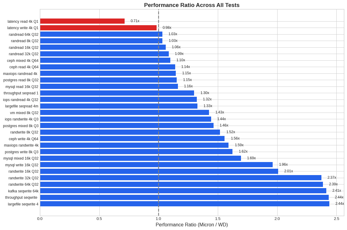
2.9 Technical Analysis
2.9.1 Why Micron Outperforms in Most Tests
Based on the benchmark data, several factors likely explain Micron’s performance advantage:
PCIe Generation / Lanes (Inference): Micron’s 2.4x sequential write advantage suggests it may be using PCIe Gen4 x4 vs Gen3 on the WD, or has superior lane utilization. The bandwidth ceiling of ~6.3 GB/s read aligns with PCIe Gen4 x4 theoretical limits.
Controller & Firmware Tuning: Micron’s remarkably consistent p99 latencies (often with stdev <100µs) indicate sophisticated garbage collection (GC) and write amplification management. WD’s high-percentile latency spikes (14ms+ in some write tests) suggest aggressive background operations or less optimized GC scheduling.
Internal Parallelism / Architecture: Despite equal capacity (14TB each), Micron appears to have higher per-die performance. This suggests more advanced NAND (possibly 176L+ TLC), more channels, or more efficient controller architecture.
Over-Provisioning: Enterprise SSDs often reserve significant spare area. Micron’s consistent sustained write performance suggests generous over-provisioning that maintains write performance as the drive fills.
Write Amplification Factor (WAF): The dramatic difference in random write IOPS (particularly at high QD) points to superior WAF management in Micron, likely through better data placement algorithms and larger write buffers.
2.9.2 Where WD 14T Excels
Low-QD Random Read Latency: WD’s p50 of 35µs vs Micron’s 71µs at QD1 random read is notable. This may indicate:
- More aggressive read path optimization
- Larger or faster DRAM cache
- Simpler FTL lookup for read operations
Capacity Economics: 14TB in a single device enables high-density deployments where raw \(/TB matters more than IOPS/\).
Read Performance Gap is Smaller: At QD32+, read performance difference narrows to 1.1-1.3x, making WD competitive for read-heavy workloads.
2.9.3 Recommendations for Our Deployment
Given our actual workload profile (~15K IOPS peak, ~800 MiB/s bandwidth, 1 PB target):
| Scenario | Recommendation | Rationale |
|---|---|---|
| Our 1 PB deployment | Tiering | SSD for hot (4-6 drives) + HDD for cold, saves ₹80L |
| Tracker (Warm 30TB) | SSD | 2-3 WD drives, 1-1.5M IOPS available |
| Tracker (Cold 120TB) | HDD | ~6 HDDs at ₹1.5K/TB = ₹1.8L |
| Domain Storage (10TB) | SSD | 1 WD drive, 505K IOPS (vs 22K needed) |
| Future growth (10x) | Still fine | Hot tier scales, cold stays on HDD |
When to reconsider Micron:
| Scenario | Threshold | Our Status |
|---|---|---|
| Single-node IOPS > 400K | Need Micron | ❌ Not needed |
| p99 latency < 500µs required | Need Micron | ❌ Not needed |
| Per-slot density critical | Consider Micron | ❌ Have rack space |
| Prefer faster writes (1.4-2.4x) | Consider Micron | ⚠️ Adds ₹0.58 Cr for 1 PB |
2.10 Conclusion
2.10.1 Key Takeaways
We are capacity-bound, not performance-bound
- Need: 1 PB storage, ~15K IOPS, ~800 MiB/s
- Single WD drive: 14 TB, 505K IOPS, 2.1 GB/s
- Ratio: Need 72 drives for capacity, but only 1 drive worth of IOPS
The Micron vs WD debate is secondary
- Both massively exceed our IOPS needs (2.4Kx headroom)
- WD saves ₹0.58 Cr for all-SSD — meaningful but not transformative
- Real savings come from questioning whether we need 1 PB of SSD at all
Tiered-HDD storage is the real opportunity
Strategy Cost Savings vs All-SSD All Micron SSD ₹1.58 Cr — All WD SSD ₹1.0 Cr ₹0.58 Cr SSD + HDD Tiering ₹18-22L ₹78-82L Recommended architecture
- Hot tier: 4-6 WD 14T SSDs (56-84 TB) for warm data + active I/O
- Cold tier: Enterprise HDDs for 900+ TB of archives/cold data
- Data movement: Time-based or access-frequency-based tiering policy
2.10.2 Final Recommendation
Action Items
Immediate: If buying SSDs now, choose WD 14T over Micron (saves ₹0.58 Cr, same performance for our needs)
Strategic: Evaluate tiered SSD+HDD architecture
- Map data access patterns (hot vs cold)
- Design tiering policy (age-based, access-frequency)
- Potential savings: ₹78-82L (vs all-SSD)
Don’t over-optimize SSD choice — the bigger lever is tiering, not Micron vs WD
2.11 Appendix A: SSD+HDD Tiering Analysis
This appendix explores the hypothesis: What if we move cold data to HDD?
2.11.1 HDD Specifications
We evaluated the Seagate 20TB SAS E-X20 enterprise HDD:
| Spec | WD 14T SSD | Seagate 20T HDD | SSD/HDD Ratio | |
|---|---|---|---|---|
| 0 | Capacity | 14 TB | 20 TB | 0.7x |
| 1 | Price | ₹1.4L | ₹34.5K | 4.1x |
| 2 | Price/TB | ₹10K | ₹1.7K | 5.8x |
| 3 | Random Read IOPS | 554K | 168 | 3,300x |
| 4 | Random Write IOPS | 505K | 350 | 1,443x |
| 5 | Seq Bandwidth | 2.1 GB/s | 285 MB/s | 7.5x |
2.11.2 Tiering Hypothesis
Assumption: In time-series/log workloads, data access follows a temporal pattern:
- Hot data (recent): ~10% of capacity, ~95% of I/O
- Cold data (old): ~90% of capacity, ~5% of I/O
2.11.3 Cost Comparison
| Configuration | Hot Tier | Cold Tier | Total Cost | Hot Tier IOPS | Cold Tier IOPS | |
|---|---|---|---|---|---|---|
| 0 | All SSD (WD 14T) | 72 SSDs (1 PB) | — | ₹101L | 36M | — |
| 1 | Tiered-HDD: SSD + HDD | 8 SSDs (100 TB) | 45 HDDs (900 TB) | ₹27L | 4.0M | 15.8K |
| 2 | Difference | — | — | **Save ₹74L** | — | — |
2.11.4 Cost Visualization

2.11.5 Can Cold Data Survive on HDD?
The critical question: Does HDD have enough IOPS for cold data?
| Scenario | Cold I/O Need | HDD Capacity (45 drives) | Headroom | Verdict | |
|---|---|---|---|---|---|
| 0 | 5% I/O on cold (baseline) | 750 IOPS | 15.8K IOPS | 21x ✅ | Comfortable |
| 1 | 10% I/O on cold | 1.5K IOPS | 15.8K IOPS | 10x ✅ | Comfortable |
| 2 | 20% I/O on cold (stress) | 3K IOPS | 15.8K IOPS | 5x ✅ | Tight but OK |
| 3 | Sequential reads (scans) | 800 MiB/s | 12.8 GB/s | 16x ✅ | Comfortable |
Answer: Yes, even with pessimistic assumptions (20% I/O on cold data), HDD provides 5x headroom.
2.11.6 Decision Matrix
| Factor | All-SSD | Tiered-HDD | Winner |
|---|---|---|---|
| Cost | ₹100L | ₹27L | Tiered-HDD (₹73L savings) |
| Hot Data IOPS | 36M | 4M | Both overkill (need 14K) |
| Cold Data IOPS | 36M | 16K | Both sufficient (need <3K) |
| Operational Simplicity | Simple | Medium | All-SSD |
| Data Movement | None | Required | All-SSD |
| Future Flexibility | Easy | More planning | All-SSD |
2.11.7 Risks and Caveats
Tiering Risks
- No middle ground: SSD → HDD is a 1,443x cliff — misclassified data will suffer
- Data classification required: Need clear hot/cold boundary (e.g., data >2 months old)
- Migration tooling: Need automated data movement between tiers
- Cold data access latency: HDD p99 is ~10-20ms vs SSD’s ~1ms
- Burst handling: If cold data suddenly becomes hot, HDD will bottleneck
Mitigation: Start conservative with 80/20 split (80% on HDD, 20% SSD buffer) to absorb classification errors.
2.11.8 Verdict
Tiering Recommendation
If cold data is truly cold (<10% I/O):
- Tiering saves ₹73L with acceptable performance
- The savings justify the added complexity of data tiering
If access patterns are unpredictable:
- Stick with all-SSD (WD 14T)
- Still saves ₹0.58 Cr vs Micron
2.12 Appendix B: Full Benchmark Results
Show code
# Create comprehensive results table
all_results = []

for test in df['test_name'].unique():
    m_row = df[(df['test_name'] == test) & (df['drive'] == 'micron_3T')]
    w_row = df[(df['test_name'] == test) & (df['drive'] == 'wd_14T')]

    if m_row.empty or w_row.empty:
        continue

    result = {
        'Test': test,
        'Workload': m_row['workload_type'].values[0],
        'QD': m_row['io_depth'].values[0],
        'M Read IOPS': f"{m_row['read_iops'].values[0]:,.0f}" if pd.notna(m_row['read_iops'].values[0]) else "-",
        'W Read IOPS': f"{w_row['read_iops'].values[0]:,.0f}" if pd.notna(w_row['read_iops'].values[0]) else "-",
        'M Write IOPS': f"{m_row['write_iops'].values[0]:,.0f}" if pd.notna(m_row['write_iops'].values[0]) else "-",
        'W Write IOPS': f"{w_row['write_iops'].values[0]:,.0f}" if pd.notna(w_row['write_iops'].values[0]) else "-",
        'M Read BW': f"{m_row['read_bandwidth_mib'].values[0]:,.0f}" if pd.notna(m_row['read_bandwidth_mib'].values[0]) else "-",
        'W Read BW': f"{w_row['read_bandwidth_mib'].values[0]:,.0f}" if pd.notna(w_row['read_bandwidth_mib'].values[0]) else "-",
        'M Write BW': f"{m_row['write_bandwidth_mib'].values[0]:,.0f}" if pd.notna(m_row['write_bandwidth_mib'].values[0]) else "-",
        'W Write BW': f"{w_row['write_bandwidth_mib'].values[0]:,.0f}" if pd.notna(w_row['write_bandwidth_mib'].values[0]) else "-",
    }
    all_results.append(result)

full_df = pd.DataFrame(all_results)
full_df| Test | Workload | QD | M Read IOPS | W Read IOPS | M Write IOPS | W Write IOPS | M Read BW | W Read BW | M Write BW | W Write BW | |
|---|---|---|---|---|---|---|---|---|---|---|---|
| 0 | latency_write_4k_qd1 | randwrite | 1 | - | - | 35,000 | 35,600 | - | - | 137 | 139 |
| 1 | latency_read_4k_qd1 | randread | 1 | 12,200 | 17,100 | - | - | 48 | 67 | - | - |
| 2 | mysql_write_16k_qd32 | randwrite | 32 | - | - | 267,000 | 136,000 | - | - | 4,166 | 2,123 |
| 3 | mysql_read_16k_qd32 | randread | 32 | 391,000 | 336,000 | - | - | 6,102 | 5,254 | - | - |
| 4 | mysql_mixed_16k_qd32 | randrw | 32 | 400,000 | 236,000 | 171,000 | 101,000 | 6,244 | 3,687 | 2,675 | 1,579 |
| 5 | postgres_write_8k_qd32 | randwrite | 32 | - | - | 432,000 | 266,000 | - | - | 3,374 | 2,076 |
| 6 | postgres_read_8k_qd32 | randread | 32 | 704,000 | 610,000 | - | - | 5,499 | 4,763 | - | - |
| 7 | postgres_mixed_8k_qd32 | randrw | 32 | 603,000 | 412,000 | 258,000 | 176,000 | 4,710 | 3,217 | 2,018 | 1,378 |
| 8 | ceph_write_4k_qd64 | randwrite | 64 | - | - | 785,000 | 504,000 | - | - | 3,068 | 1,969 |
| 9 | ceph_read_4k_qd64 | randread | 64 | 1,146,000 | 1,006,000 | - | - | 4,475 | 3,931 | - | - |
| 10 | ceph_mixed_4k_qd64 | randrw | 64 | 853,000 | 776,000 | 366,000 | 333,000 | 3,332 | 3,031 | 1,428 | 1,299 |
| 11 | vm_mixed_8k_qd32 | randrw | 32 | 537,000 | 376,000 | 289,000 | 203,000 | 4,195 | 2,941 | 2,259 | 1,584 |
| 12 | kafka_seqwrite_64k | write | 16 | - | - | 82,100 | 34,000 | - | - | 5,132 | 2,124 |
| 13 | iops_randwrite_4k_qd32 | randwrite | 32 | - | - | 729,000 | 505,000 | - | - | 2,847 | 1,971 |
| 14 | iops_randread_4k_qd32 | randread | 32 | 733,000 | 554,000 | - | - | 2,864 | 2,163 | - | - |
| 15 | maxiops_randwrite_4k_qd128 | randwrite | 128 | - | - | 786,000 | 494,000 | - | - | 3,069 | 1,929 |
| 16 | maxiops_randread_4k_qd128 | randread | 128 | 1,138,000 | 993,000 | - | - | 4,445 | 3,878 | - | - |
| 17 | throughput_seqwrite_1m | write | 32 | - | - | 5,204 | 2,137 | - | - | 5,204 | 2,137 |
| 18 | largefile_seqwrite_4m | write | 16 | - | - | 1,298 | 532 | - | - | 5,196 | 2,131 |
| 19 | largefile_seqread_4m | read | 16 | 1,583 | 1,192 | - | - | 6,333 | 4,768 | - | - |
| 20 | randwrite_8k_qd32 | randwrite | 32 | - | - | 404,000 | 266,000 | - | - | 3,159 | 2,082 |
| 21 | randread_8k_qd32 | randread | 32 | 619,000 | 599,000 | - | - | 4,838 | 4,677 | - | - |
| 22 | randwrite_16k_qd32 | randwrite | 32 | - | - | 267,000 | 133,000 | - | - | 4,171 | 2,079 |
| 23 | randread_16k_qd32 | randread | 32 | 386,000 | 364,000 | - | - | 6,026 | 5,692 | - | - |
| 24 | randwrite_32k_qd32 | randwrite | 32 | - | - | 159,000 | 67,000 | - | - | 4,961 | 2,093 |
| 25 | randread_32k_qd32 | randread | 32 | 213,000 | 196,000 | - | - | 6,643 | 6,120 | - | - |
| 26 | randwrite_64k_qd32 | randwrite | 32 | - | - | 80,200 | 33,600 | - | - | 5,014 | 2,100 |
| 27 | randread_64k_qd32 | randread | 32 | 102,000 | 98,900 | - | - | 6,397 | 6,181 | - | - |
| 28 | throughput_seqread_1m | read | 32 | 6,306 | 4,850 | - | - | 6,307 | 4,850 | - | - |
2.13 Appendix C: Data Sources
This report was generated from the following data files:
| File | Description |
|---|---|
| fio_comparison.csv | Raw fio benchmark results for Micron and WD SSDs |
| Server - AWS Instance Distribution - IO Throughput Across Clusters.csv | Production cluster I/O throughput data |
| db-traffic.png | Database traffic requirements visualization |
2.13.1 Storage Pricing Used
| Device | Capacity | Price | Source |
|---|---|---|---|
| Micron 14T NVMe SSD | 14 TB | ₹2.2L | Vendor quote |
| WD 14T NVMe SSD | 14 TB | ₹1.4L | Vendor quote |
| Seagate E-X20 HDD | 20 TB | ₹34.5K | Vendor quote |
Report generated from fio benchmark data. Model numbers not provided in source data. Performance inferences marked accordingly.